Pipelines to simulate and detect indels

This post describes a pipeline to simulate short reads using wgsim, align the produce short reads using BWA or Bowtie2 and finally detects indels using GATK UnifiedGenotyper (Broad Institute) or Dindel (Welcome Trust Sanger Institute).

Step 1 - Get a reference genome

I chose to get the human reference genome v37 from 1000 Genomes Project: download link to human_g1k_v37.fasta.gz file (851MB). You can extract the chromosome of your choice (to avoid working on the whole genome) with samtools:

samtools faidx human_g1k_v37.fasta 20 > human_g1k_v37_chr20.fasta


Step 2 - Simulate short reads

There are several short reads simulators (e.g. MAQ, SimSeq, FluxSimulator). Here we are going to use wgsim that was once included in samtools and later extracted as a standalone project.

Wgsim project homepage: https://github.com/lh3/wgsim

Before running the simulator we need to calculate the number of reads we need. Remember the formula to calculate the coverage:

Coverage = N x L / G

(where N: number of reads - L: read length - G: genome size)

To detect indels we aim to have a "good" coverage of the genome, let's aim to get a coverage around 20. Then, if we produce 70-bp reads on human chromosome 20 (63Mbp long), it is easy with the formula above to find that we need at least 18.000.000 reads to achieve this coverage.

Once installed one run wgsim with the following command to generate the two files of paired reads:

wgsim -N 20000000 -X 0.95 human_g1k_v37_chr20.fasta out.read1.fq out.read2.fq > wgsim.out


Note the use of the -X option to increase the probability to extend an indel. The file wgsim.out will contain the indels generated where the column 1 is the chromosome, column 2 is the position, column 3 is the original base, column 4 is the new base (following the IUPAC codes) and column 5 is genomic copy/haplotype. The files out.read1.fq and out.read2.fq will contains the two reads of the paired reads (remember we are working with PEM here).

A limitation of wgsim is that it generates bases with a fixed quality of Q17 (encoded as "2" in fastq file) and the UnifiedGenotyper to be used below throws away everything that is below Q20. Hence we can reprocess the fastq files to uniformly increase base qualities with a awk command (Credit: biostar contribution):

awk ' /222/ { gsub("2", "I"); print $0; next } { print } ' out.read1.fq > out.read1b.fq
awk ' /222/ { gsub("2", "I"); print $0; next } { print } ' out.read2.fq > out.read2b.fq

Step 3 - Aligning short reads
Whatever the alignment method you choose, be sure to apply "Post-processing of alignment file" before going ahead with next step.

3.1. Aligning using BWA
Please consult BWA Manual Reference pages to get more details on the commands used below to index database sequences in the FASTA format (index), Find the SA coordinates of the input reads (aln), and finally generate alignments in the SAM format given paired-end reads (sampe):

bwa index human_g1k_v37_chr20.fasta

Important: the default BWA algorithm for constructing index, IS, is fast but will not work on database (fasta file) larger than 2GB. For larger database, use the option "-a bwtsw". 

bwa aln human_g1k_v37_chr20.fasta out.read1b.fq -f out1.sai
bwa aln human_g1k_v37_chr20.fasta out.read2b.fq -f out2.sai


Note: if your computer has several CPUs, you probably want to use them all through the "-t" option (see BWA Manual Reference pages). 

bwa sampe -f out.sam -r '@RG\tID:foo\tSM:bar' human_g1k_v37_chr20.fasta out1.sai out2.sai out.read1b.fq out.read2b.fq
samtools view -hbS out.sam -o out.bam 

Note:  as an optimization the command "bowtie2..." could be pipedto the "samtools view..." command in order to generate directly the binary version of the alignment file (.bam instead of .sam) and avoid the creation of an intermediary .sam file. This is an optimization proposed by swbarnes2 in SEQanswers.

Note: as suggested by Heisman in SEQanswers, the previous command may also be optimized using the optional parameter -u to request samtools not to compress the .BAM file as this will be done by the "samtools sort" command below.

3.2. Aligning using Bowtie
As an alternative to BWA, we can use Bowtie 2 to align short reads to the genome. First, call bowtie-build to index our reference genome:

bowtie2-build human_g1k_v37_chr20.fasta homo_chr20

Then the call to actually create the alignment:

bowtie2 -t homo_chr20 -X 700 -1 out.read1b.fq -2 out.read2b.fq -S out.sam
samtools view -hbS out.sam -o out.bam

Note: as an optimization the command "bowtie2..." could be pipedto the "samtools view..." command in order to generate directly the binary version of the alignment file (.bam instead of .sam) and avoid the creation of an intermediary .sam file. This is an optimization proposed by swbarnes2 in SEQanswers.

Note: as suggested by Heisman in SEQanswers, the previous command may also be optimized using the optional parameter -u to request samtools not to compress the .BAM file as this will be done by the "samtools sort" command below.

3.3. Post-processing of alignment file
Before calling indels, the alignment file will be converted in binary format, sorted then indexed using samtools:

samtools sort out.bam out_sorted
samtools index out_sorted.bam

Step 4 - Calling indels

4.1. Calling indels with GATK UnifiedGenotyper

Important: running the local realignment as described here is highly recommended to improve accuracy prior to run UnifiedGenotyper.

java -jar /home/pmaugeri/tools/GenomeAnalysisTK-1.3-21-gcb284ee/GenomeAnalysisTK.jar -R human_g1k_v37_chr20.fasta -T UnifiedGenotyper -I out_sorted.bam -o gatk_indels.vcf -glm INDEL

Indels called by the UnifiedGenotyper can be found in the file specified by the -o option (file "gatk_pipeline_indels.vcf").

Here's an example of a VCF file generated with GATK with this pipeline: gatk.vcf (~2MB)

4.2. Calling indels with Dindel
Calling indels using Sanger software is done in 4 steps where the first and the third are the longest ones:

dindel --ref human_g1k_v37_chr20.fasta --outputFile 1 --bamFile out_sorted.bam --analysis getCIGARindels

python makeWindows.py --inputVarFile 1.variants.txt --windowFilePrefix 2 --numWindowsPerFile 20000

dindel --analysis indels --doDiploid --bamFile out_sorted.bam --ref human_g1k_v37_chr20.fasta --varFile 2.1.txt --libFile 1.libraries.txt --outputFile 3 > 3.out 2> 3.err

echo 3.glf.txt > 3.list
python mergeOutputDiploid.py -i 3.list -o dindel_indels.vcf -r human_g1k_v37_chr20.fasta

Indels called by Dindel are found in file specified by -o option.

Here's an example of a VCF file generated with Dindel with this pipeline: dindel.vcf (~300KB)


Thanks a lot to Alex Renwick, swbarnes2, Heisman and vyellapa for their great suggestions in   SEQanswers forum to improve this post.

Genome Structural Variation on simulated genome

Here's a brief memo to simulate a read alignment (and indels) based on a human genome chromosome and detect Structural Variations.


Step 1 - Get a reference genome

I chose to get the human reference genome v37 from 1000 Genomes Project: download link to human_g1k_v37.fasta.gz file (851MB).

You can extract the chromosome of your choice (to avoid working on the whole genome) with samtools:

samtools faidx human_g1k_v37.fasta 20 > human_g1k_v37_chr20.fasta

Step 2 - Simulate reads and indels

There are several short reads simulators (e.g. SimSeq, FluxSimulator). Here we are going to use wgsim that was once included in samtools and later extracted as a standalone project.

Wgsim project homepage: https://github.com/lh3/wgsim

Before running the simulator we need to calculate the number of reads we need. Remember the formula to calculate the coverage:

Coverage = N x L / G

(where N: number of reads - L: read length - G: genome size)

To detect indels we aim to have a "good" coverage of the genome, let's aim to get a coverage around 20. Then, if we produce 70-bp reads on human chromosome 20 (63Mbp long), it is easy with the formula above to find that we need at least 18.000.000 reads to achieve this coverage.

Once installed you run wgsim with the following command to generate the two files of paired reads:

wgsim -N 20000000 -X 0.95 human_g1k_v37_chr20.fasta out.read1.fq out.read2.fq > wgsim.out

Note the use of the -X option to increase the probability to extend an indel. The file wgsim.out will contain the indels generated where the column 1 is the chromosome, column 2 is the position, column 3 is the original base, column 4 is the new base (following the IUPAC codes) and column 5 is genomic copy/haplotype. The files out.read1.fq and out.read2.fq will contains the two reads of the paired reads (remember we are working with PEM here).

Step 3 - create the alignment file
With the paired reads files created in previous files we can align these reads against the reference genome and create an alignment file.

Again here, several tools are available and we will use bowtie2.

First, call bowtie-build to index our reference genome

bowtie2-build human_g1k_v37_chr20.fasta homo_chr20


Then the call to actually create the alignment:

bowtie2 -t homo_chr20 -X 700 -1 out.read1.fq -2 out.read2.fq -S homo_chr20.sam

Convert the alignment file to a binary alignment file (.SAM -> .BAM), sort and index using samtools:

samtools view -bS homo_chr20.sam > homo_chr20.bam
samtools sort homo_chr20.bam homo_chr20_sorted
samtools index homo_chr20_sorted.bam

Step 4 - detect Structural Variants
The following command calls shows how to detect indels generated in step 1:

dindel --ref human_g1k_v37_chr20.fasta --outputFile 1 --bamFile homo_chr20_sorted.bam --analysis getCIGARindels

python makeWindows.py --inputVarFile 1.variants.txt --windowFilePrefix 2 --numWindowsPerFile 20000

dindel --analysis indels --doDiploid --bamFile homo_chr20_sorted.bam --ref human_g1k_v37_chr20.fasta --varFile 2.1.txt --libFile 1.libraries.txt --outputFile 3 > 3.out 2> 3.err

echo 3.glf.txt > 3.list

python mergeOutputDiploid.py -i 3.list -o 4.vcf -r human_g1k_v37_chr20.fasta

Using XSL to filter biomedical data

This post gives a short introduction to XSLT (for Extended Stylesheet Language Transformation) that will be used to transform an XML file into something else. This something else could be another XML file with a different structure, a CSV file or any other text content.

This is a very tiny tutorial intended to help you in setting your environment and doing a first transformation using biomedical data, so I won't go into details of the language nor try to provide an exhaustive list of available operations, there is already plenty of good literature and reference on this subject (see last paragraph "Further reading").

I used this technology some years ago to dynamically transform a stream of data into either a HTML page or a WAP page (for mobile phone internet browser) depending on the client being detected. But here we are going to use XSL for handling and transforming a XML document resulting from a search in UniProt (list of proteins).

Objective: let's say we want to transform the XML document downloaded from UnitProt into a nicer CSV file with two columns: the protein name and the gene name.

You will see that the corresponding filter could be easily adapted to your needs or to any other biomedical source of data (MeSH, Drugbank, etc.).

Requirements/Environment
In order to run XSL in your computer you need the following software installed and properly configured:

• Java 1.6 or higher
• Download and install xalan-j_2_7_1-bin
• once you have Xalan installed, define the environment variable XALAN_HOME that will point to Xalan root folder (e.g. XALAN_HOME=C:\java\xalan-j_2_7_1)
• update your Java classpath, it should at least include:
  
  CLASSPATH=%XALAN_HOME%\xalan.jar;%XALAN_HOME%\xalan.jar;%XALAN_HOME%\serializer.jar;%XALAN_HOME%\xml-apis.jar;%XALAN_HOME%\xercesImpl.jar

Input data

We will use the XML data produced by UniProtKB when searching for proteins related to organism "Moloney murine leukemia virus". This is random example to demonstrate the technique on a small XML file, but of course the same could be applied on different data.

Follow these steps to get the XML file:

1. go to http://www.uniprot.org
2. run a search using the query:
   organism:"Moloney murine leukemia virus"
3. in the search result page click the Download link
4. download the file "Complete Data in XML format" and save it using the filename uniprot.xml

So we have a XML file to play with. You may open it in a text editor to understand the structure of the XML content before doing the XSL script. Note that Uniprot returned around 22 proteins, so you should find in the XML file 22 <entry/> blocks

Write your XSL script

We will write a simple XSL script that will output 2 columns of data: a column with the "Protein fullname" and a column with the "Gene name". Both columns will be separated with a TAB character.

Open a text editor and create a file uniprot.xsl.

A XSL script is itself an XML file! So it should logically start by the header:

<?xml version="1.0" encoding="ISO-8859-1"?>

Then the whole XML document should be written between the "stylesheet" tag:

<xsl:stylesheet version="1.0" xmlns:xsl="http://www.w3.org/1999/XSL/Transform">

...

</xsl:stylesheet>

The next line will say to the XSL interpreter to match the root of the XML document:

<xsl:template match="/">

Then this prints the column header of our CSV file (a TAB between two headers and a line feed character at the end):

<!-- Print columns headers -->

<xsl:text>Accession</xsl:text>

<xsl:text>&#x9;</xsl:text>

<xsl:text>Gene name</xsl:text>

<xsl:text>&#10;</xsl:text>

The following block is a bit more sophisticated. It is a loop on each "entry" tag of your XML file. For each entry it will print the full name of the protein (follow the XML path), and the gene name:

<xsl:for-each select="uniprot/entry">

<xsl:value-of select="accession"/>

<xsl:text>&#x9;</xsl:text>

<xsl:value-of select="gene/name"/>

<xsl:text>&#x9;</xsl:text>

<xsl:text>&#10;</xsl:text>

</xsl:for-each>

For your convenience here is the complete XSL file content:

<?xml version="1.0" encoding="ISO-8859-1"?>

<xsl:stylesheet version="1.0" xmlns:xsl="http://www.w3.org/1999/XSL/Transform">

<xsl:template match="/">

<!-- Print columns headers -->

<xsl:text>Accession</xsl:text>

<xsl:text>&#x9;</xsl:text>

<xsl:text>Gene name</xsl:text>

<xsl:text>&#10;</xsl:text>

<xsl:for-each select="uniprot/entry">

<xsl:value-of select="accession"/>

<xsl:text>&#x9;</xsl:text>

<xsl:value-of select="gene/name"/>

<xsl:text>&#x9;</xsl:text>

<xsl:text>&#10;</xsl:text>

</xsl:for-each>

</xsl:template>

</xsl:stylesheet>

Run your XSL script

Once you have your input XML and your XSL written, you are ready to try it. The following will parse the input XML file and output the desired data defined previously in CSV file that you may us in Excel:

java org.apache.xalan.xslt.Process -IN uniprot.xml -XSL uniprot.xsl -OUT uniprot.csv

Tip: remember that if you manipulate large XML file, your Java runtime may complain about the heap space. You can increase the heap space by adding the parameter -Xms to the java command line.

Further reading:

• http://www.w3schools.com/xsl/default.asp
• What is XSLT?

Development of Drugs in Public-Private Partnerships environments

This week we organized a debate about the Development of Drugs in Public-Private Partnerships (PPP) environments. It raised some passionate interventions by the participants.

Here are the slides we used to introduce this subject. We are using Orphan Diseases as a potential field where PPP could be fruitful and we present the project Grants4Targets as an example of PPP.

If you are looking for data for your market research on drug development I suggest you have a look to the References slide (slide #18), it contains interesting materials.

Recommended book

I have recently read "Molecular Modeling: Basic Principles and Applications". It gives a very good introduction for Structural Bioinformatics and also some bits of information for Molecular Simulation. It is a small, light and clearly written book.

[ Wiley | Amazon ]

The new chapter "Chemogenomic Approaches to Rational Drug Design" has been added to the third edition (I have actually read the second one).

Table of contents:

1. Introduction.
2. Small Molecules.
3. A Case Study for Small Molecule Modeling: Dopamine D3 Receptor Antagonists.
4. Introduction to Comparative Protein Modeling.
5. Virtual Screening and Docking.
6. Scope and Limits of Molecular Docking.
7. Chemogenomic Approaches to Rational Drug Design.
8. A Case Study for Protein Modeling: the Nuclear Hormone Receptor CAR as an example for Comparative Modeling and the Analysis of Protein-Ligand Complexes.

Structural introduction to HLA/MHC

An introduction to HLA protein group giving some nice pictures on structures of HLA/MHC.

Here are some pictures from the slideset:

View of a peptide binding site of MHC Class-I (HLA-B27, PDB: 1HSA)

MHC HLA-A2 (in blue) bound to TCR (in red)

Visit of Parc Cientific Barcelona

Today, I had the great opportunity to visit Parc Cientific Barcelona. A great cocktail of biomedicine labs and companies. It shows Catalunya is investing hard in the sector.

The labs are cleaned, well organized and equiped with brand new equipments.

Some pictures of the "tour" here...

In the basement, some zebra fishes waiting for being fished by lab technicians (there were also a bunch of frogs behind :->):

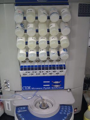
a peptide synthetizer (?):

An old "electron microscope" was waiting for its turn to go to museum:

Fixing errors in a model

Here is an interesting exercice (and solution) we did today in Structural Bioinformatics class.

The goal is to fix an error in the following model:

Did you see this loop in the middle of the alpha-helix ?!

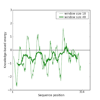
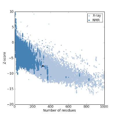
Before fixing it, these are Prosa plots of this model which confirm the error:

So here are the steps we followed to fix it. There are also interesting tricks to know to manipulate the data.

Getting the Amino Acids sequence

In order to get the corresponding AA sequence out of the PDB file, we simply splitted the PDB using our local tool which also generates the FASTA file out of PDB:

PDBtoSplitChain.pl -i wrong-model.pdb

You may also use this public tool: Make sequence file from PDB file

Prepare the alignment for modeler

Then we produced an alignment between our target sequence against itself:

cat wrong-model.fa > homologs.fa

cat wrong-model.fa >> homologs.fa

Edit the homologs.fa file and name the first sequence "seq" and the second "model".

Create a clustal alignment with homologs.fa

clustalw homologs.fa

(or do it online through http://www.ebi.ac.uk/Tools/msa/clustalw2/)

We have to locate the error (the loop of the alpha helix) in this alignment. For that purpose, we used Jmol and doing clicks on the AA of the loop we found the sequence Serine->Serine->Valine->Glutamic->Glutamic->Leucine->Leucine or ...SSVEELL...

We edit the alignment file and shift this subsequence to the right:

seq [...]QVAKSSVEELLLSQNSVKSL

model [...]QVAKSSVEELLLSQNSVKSL

Becomes:

seq [...]QVAKSSVEELLLSQNSVKSL-------

model [...]QVAK-------SSVEELLLSQNSVKSL

With this alignment we can produce a new model.

Generate a better model

Based on the alignment modified in previous section, we are going to produce a model and assess whether we improve it or not.

Convert the Clustal alignment file into a PIR file.

For that purpose you may try the online tool: Sequence Format Converter.

With the alignment in PIR format ready prepare the Modeler script:

from modeller import * # Load standard Modeller classes

from modeller.automodel import * # Load the automodel class

log.verbose() # request verbose output

env = environ() # create a new MODELLER environment to build this model in

# directories for input atom files

env.io.atom_files_directory = ['.', '../atom_files']

a = automodel(env,

alnfile = 'homologs.ali', # alignment filename

knowns = ('seq'), # codes of the templates

sequence = 'model') # code of the target

a.starting_model= 1 # index of the first model

a.ending_model = 3 # index of the last model

# (determines how many models to calculate)

a.make() # do the actual homology modeling

and create the model:

mod9v7 model-default.py

Assessment of the new model

This is the new model we just produced. Observed that the loop does not appear in the alpha helix:

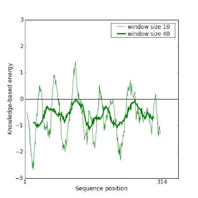
And indeed this new model gives a much better result in Prosa:

This manual modification of the alignment can be iteratively done to improve even more the model.

Calculating distances with VMD Tk scripting

This post shows how to calculate distances between atoms using Tk scripting.

Assuming you have loaded the molecule 1NEY in VMD we are going to calculate the distance between the atom OE1 of chain A with all of the residues of the protein. We will consider the alpha-Carbon atom to be arbitrary the center of a residue.

Open the Tk Console with menu Extensions > Tk Console.

The following two lines store the coordinates of oxygen named OE1:

% set oe1 [atomselect top "name OE1 and resid 165 and chain A"]
% set OE1coord [lindex [$oe1 get {x y z}] 0]

This will store all alpha-Carbon carbons in the list CASel:

% set CASel [atomselect top "type CA"]

Then to compute the distance between OE1coord an each element of CASel, you just run this script:

% foreach ca [$CASel get {x y z}] {

set distance [veclength [vecsub $OE1coord $ca]]

echo $ca : $distance

}

Displaying protein chains with VMD

VMD is a molecular visualization program that can display static or animated systems. It has a built-in programming language called Tk. The version used in this post is 1.8.7.

We are going to show some common operations on the protein Triosephosphate Isomerase in Complex with DHAP using this modified PDB file.

We start by displaying the protein chains using different colors.

1. start VMD program
2. menu File > New Molecule, browse to the downloaded file 1NEY.pdb, then click Load button. You should see something like this:
   
   
   
3. menu Graphics > Representations
4. select the line in the list of representations and delete it by clicking Delete Rep button,
5. click twice the Create Rep button to create one graphical representation for each chain,
6. select the first graphical representation line,
   - for Drawing Method choose for instance NewRibbons
   - for Coloring Method choose ColorID and then choose a color in the list of IDs
   - in the Selected Atoms field enter chain A
   - then click the button Apply
7. select the second graphical representation line,
   - for Drawing Method choose for instance NewRibbons
   - for Coloring Method choose ColorID and then choose another color in the list of IDs
   - in the Selected Atoms field enter chain B
   - then click the button Apply

You should get this output:

Remember the keyboard shortcuts to toggle the mouse pointer mode:

• r for rotating
• t for translating
• s for scaling

Python and Doxygen

Dogygen produces a professional documentation of your source code. Originally wrote for C/C++ source code, it now supports a broader range of language: C, C++, Java, PHP, Python, etc.

Here is a quick howto to get your Python project documented:

1. download a binary distribution and install it in your system
   
   
2. generate a configuration file template running in a command line console:
   
   doxygen -g my_project.doxyfile
   
   
3. update the configuration template to match your project folder, and options. So far I have configured the following options only:
   
   PROJECT_NAME
   PROJECT_NUMBER
   OUTPUT_DIRECTORY (where you want the documentation files to be written)
   EXTRACT_ALL = YES
   EXTRACT_PRIVATE = YES
   EXTRACT_STATIC = YES
   FILE_PATTERNS = *.py
   RECURSIVE = YES
   GENERATE_LATEX = NO
   
   
4. then simply run doxygen with the configuration file as parameter:
   
   doxygen my_project.doxyfile

Here's some HTML output:

Adding Biopython dependency to your Python project in Eclipse

This short post helps you to configure your Python project in Eclipse to use of biopython library.

First, you have to install separately NumPy (biopython required dependency) and biopython itself as explained in the biopython installation help.

Then, in Eclipse, open your Python project properties (Alt+ENTER when the project is selected).

Select the section PyDev - PYTHONPATH, then the tab External Libraries and make sure you have the source folder '...\site-packages' (or any other root folder you may have chosen to install Biopython). You should get the following screen:

Then you should be able to run a program such as the following:

parser = PDBParser()

structure = parser.get_structure("2BEG", "C:\\svn\\sporna\\2BEG.pdb")

for atom in structure.get_atoms():

print atom.get_name(), " coord:", atom.get_coord()

Tested on:

• Eclipse Helios Service Release 1
• Python 2.7
• Numerical Python library (NumPy) v1.5.1
• Biopython v1.56

Jmol applet (quick) howto

Here is a short post to include Jmol rendering in your blogger posts.

First of all, you need to have the applet and its related jar and resources files available somewhere behind a HTTP server. In my configuration I have a folder called JmolFolder with these 19 files:

JmolApplet0_Console.jar

JmolApplet0.jar

JmolApplet0_Minimize.jar

JmolApplet0_Popup.jar

JmolApplet0_ReadersCifPdb.jar

JmolApplet0_ReadersMolXyz.jar

JmolApplet0_ReadersMore.jar

JmolApplet0_ReadersQuantum.jar

JmolApplet0_ReadersSimple.jar

JmolApplet0_ReadersXml.jar

JmolApplet0_ReadersXtal.jar

JmolApplet0_ShapeBio.jar

JmolApplet0_ShapeSpecial.jar

JmolApplet0_ShapeSurface.jar

JmolApplet0_Smiles.jar

JmolApplet0_Symmetry.jar

JmolApplet.jar

Jmol.jar

Jmol.js

Note that I removed all the internationalization files from the original distribution (I hope it makes it start faster).

In blogger/blogspot post you have to insert the following as HTML:

<form>
<script src="http://biotechies.site40.net/jmol/JmolFolder/Jmol.js" type="text/javascript"></script> <script type="text/javascript"> jmolInitialize("http://biotechies.site40.net/jmol/JmolFolder"); jmolApplet(400, "load http://biotechies.site40.net/jmol/alphahelix.pdb.gz;");jmolBr();</script>
</form>

The result is:

First protein modeled

Also this post is not rocket-science, here is my firt protein modeled by Homology modeling. I tried to describe in details the process followed here.

First of all, this the FASTA sequence of the protein to be modeled:

>sequence   DLWNAIDPAIIADDHGQVWMSFGSFWGGLKLFKLNDDLTRPAEPQEWHSIAKLERSVLMDDSQAGSAQIEAPFILRKGDYYYLFASWGLCCRKGDSTYHLVVGRSKQVTGPYLDKTGRDMNQGGGSLLIKGNKRWVGLGHNSAYTWDGKDYLVLHAYEAADNYLQKLKILNLHWDGEGWPQVDEKELDSYIQVDVHDPVMTREGDTWYLFSTGPGITIYSSKDRVNWRYSDRAFATEPTWAKRVSPSFDGHLWAPDIYQHKGLFYLYYSVSAFGKNTSAIGVTVNKTLNPASPDYRWEDKGIVIESVPQ

Selecting homologs

I picked up the following homologs from a from a search result of the sequence with blastp:

• 1GYD_B
• 1GYH_D
• 1WL7_A

Note that those are chain of proteins. For each of them, I donwloaded the corresponding protein .pdb file (1GYD.pdb, 1GYH.pdb, 1WL7.pdb from PDB.

Then I splitted the chains from the PDB file. Here we use a homemade Perl script called PDBtoSplitChain.pl but I guess you may use splitpdb also. This will generate a file for each chain found in the PDB file.

Multiple Sequence Alignment of the homologs

Then we concatenate all the selected chains into the same file to run a MSA:

$ cat sequence.fa > homologs.fa

$ cat 1GYDB.fa >> homologs.fa

$ cat 1GYHD.fa >> homologs.fa

$ cat 1WL7A.fa >> homologs.fa

$ cat 3C2UA.fa >> homologs.fa

$ clustalw homologs.fa

The output file of clustaw (*.aln file) should be converted to a PIR file:

$ aconvertMod2.pl -in c -out p <homologs.aln >homologs.ali

Creation of the model

We are going to use Modeller 9v7 to create our model.

First the python script model-default.py for Modeller is edited:

from modeller import *

from modeller.automodel import *

log.verbose()

env = environ()

env.io.atom_files_directory = ['.', '../atom_files']

a = automodel(env,

alnfile = 'homologs.ali',

knowns = ('1GYDB', '1GYHD', '1WL7A'),

sequence = 'sequence')

a.starting_model= 1

a.ending_model = 1

a.make()

And the model is actually calculated with the following:

$ mod9v7 model-default.py

In case of error, check out the file model-default.log that is produced in the current directory.

Alignment of protein sequences based on 3D structure (STAMP)

We need to create a file called (for instance) domains.data referencing the domains of our template proteins plus the model we've just calculated in the previous step:

./1GYDB.pdb 1GYDB {all}

./1GYHD.pdb 1GYHD {all}

./1WL7A.pdb 1WL7A {all}

./sequence.B99990001.pdb mod1 {all}

Then we run stamp to superpose our model with the template proteins:

$ stamp -n 2 -rough -prefix sequence -f domains.dat

$ transform -f sequence.3 -g -o sequence.3.pdb

Nota Bene: with transform use the file sequence.[number] with the highest [number] generated by stamp (it depends on the set of sequences you used in model-default.py)

Here is a graphical rendering with Jmol of the superposition (you can move the model using drag n' drop, or use Jmol contextual menu with right click):